How Long Should You Test a Trading Strategy?

Testing a trading system involves evaluating its performance over a certain period of time and under various market environments. 

The length of the testing period can significantly impact the results and confidence in the system. 

Several key variables go into determining how long to test a trading strategy or system.

It really boils down to:

• What is the trading strategy’s edge?
• What is its frequency?
• What’s its payout?

And go into 10 separate categories of consideration.

Key Takeaways – How Long to Test a Trading Strategy

• Test Across Market Conditions
  • Be sure your strategy is tested in diverse market environments (bull, bear, volatile) to gauge robustness.
• Sufficient Trade Sample Size
  • The more trades, the more statistically significant your results.
  • 3 main variables – edge, frequency, payout 
  • Low-frequency systems with lower edges and lower payouts need longer periods.
• Monte Carlo Simulations
  • Monte Carlo simulations can be used as exercises to estimate how long it takes for your trading edge to manifest, considering randomness and variance.
• Factor in Real-World Costs
  • Include execution costs, liquidity constraints, and market impact in your testing to ensure realistic results.
• Avoid Overfitting
  • Test with out-of-sample data and use walk-forward analysis to confirm that your strategy is genuinely robust.
• Depends on the Type of Strategy
  • Given practical considerations, years and decades of backtesting generally makes sense for longer-term trading strategies (e.g., position trading, investing).
  • For shorter-term strategies where there is lots of data and trials (e.g., HFT or market making in highly liquid markets or some day trading applications), a shorter time horizon may be sufficient.

Edge, Frequency, Payout

A successful trading strategy hinges on three main variables: Edge, Frequency, and Payout.

Edge

Edge refers to the advantage a strategy has in the market, usually expressed as the probability of winning a trade.

Even a small edge, like winning 51% of the time, can be profitable over many trades.

Nonetheless, it depends on the expected value of the trade.

A 51% win rate can be great when the reward is equal to or greater than the penalty for being wrong, but be unfavorable when the penalty is greater than the reward.

Frequency

Frequency indicates how often the strategy trades.

High-frequency strategies can capitalize on small edges more quickly, as the sheer number of trades allows the edge to manifest over time.

Conversely, low-frequency strategies need a more significant edge or better payouts to be effective.

Payout

Payout is the average reward-to-risk ratio of each trade.

A high payout means that the profits from winning trades significantly exceed the losses from losing trades.

Even with a modest edge or lower frequency, a high payout can make a strategy profitable.

Balance of the Three

Balancing these three variables is key.

A strategy with a small edge might still succeed if it trades frequently or has a high payout.

A strategy with a low frequency of signals can still be good if it has a large edge and quality payout.

And a low payout strategy can be worth pursuing if the edge is higher and there are larger signal frequencies.

But overall, understanding and optimizing edge, frequency, and payout ensures that your strategy is robust and capable of generating consistent returns.

Monte Carlo Simulations of How Long It Takes a Trading Edge to Show Up

First, let’s start off with some Monte Carlo simulations.

These can be a great technique to understand how long it might take for a trading edge to become apparent.

By simulating thousands of possible outcomes based on your trading edge (the probability of winning and the average amount won or lost per trade), you can observe how the balance of your trading account evolves over time.

In this context, the trading edge, bet size, and number of trades are all critical variables. 

The edge reflects the slight advantage (or disadvantage) you have in each trade, while the bet size determines the financial impact of each trade. 

The number of trades simulates the trade frequency and passage of time in the market.

By running these simulations, you can see how long it typically takes for the cumulative profits to outweigh the natural variance in results. 

Even with a positive edge, the outcome of each trade is subject to randomness, so it may take many trades before the edge becomes statistically significant. 

The Monte Carlo approach helps you estimate the range of outcomes and understand the patience required for a trading edge to manifest in real trading conditions.

Code

We have 3 variables:

• win and loss probability
• bet amount ($100 per trade in this case)
• trials (trades/passage of time)

Here’s our code:

import numpy as np

import matplotlib.pyplot as plt

# Parameters

win_prob = 0.501 # Probability of winning

lose_prob = 0.499 # Probability of losing

bet_amount = 100 # Amount bet per round

trials = 10000 # Number of trials/trades – i.e., passage of time

# Monte Carlo sim

def monte_carlo_simulation(trials, win_prob, lose_prob, bet_amount):

# Simulate the outcomes of each trial (1 for win, -1 for loss)

outcomes=np.random.choice([1, -1], size=trials, p=[win_prob, lose_prob])



# Calculate the result of each bet

results=outcomes*bet_amount



# Calculate the cumulative sum of results to track the balance over time

balance=np.cumsum(results)



returnbalance

# Run the sim

balance = monte_carlo_simulation(trials, win_prob, lose_prob, bet_amount)

# Plot

plt.figure(figsize=(10, 6))

plt.plot(balance)

plt.title("Monte Carlo Simulation of Trading System with 50.1% Edge")

plt.xlabel("Number of Bets")

plt.ylabel("Cumulative Balance ($)")

plt.grid(True)

plt.show()

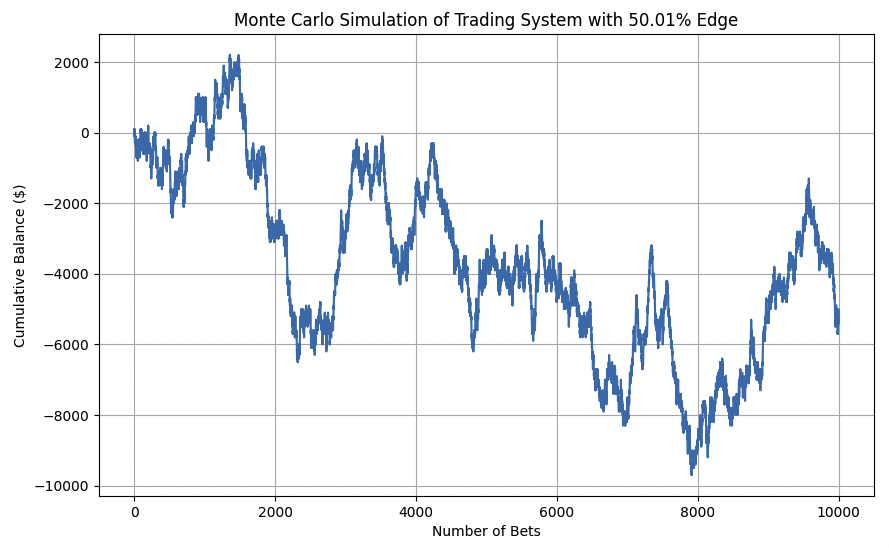
50.01% Edge

We can see with a 50.01% edge, it’s so small that it’s not much different than operating with no edge.

There’s a bit more than a 50% chance of making money over 10,000 trades, but it could very well swing the other way as it did here.

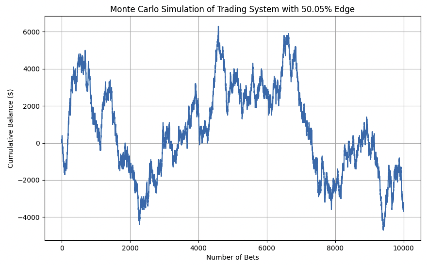
50.05% Edge

50.05% edge displays a better but similar pattern where over enough trials you can still be in the red.

Over 100,000 trials it will very likely be in the black, but the edge is so slight that variance can win out over short- and medium-term time horizons.

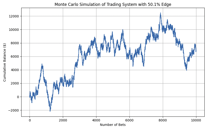
50.1% Edge

A 50.1% edge has lots of variance still, but 50.1% represents enough to skill to get ahead over 10,000 trades.

In this simulation, we were up about $7,000 (using the $100 win/loss bet size), or eking out just $0.70 per trade.

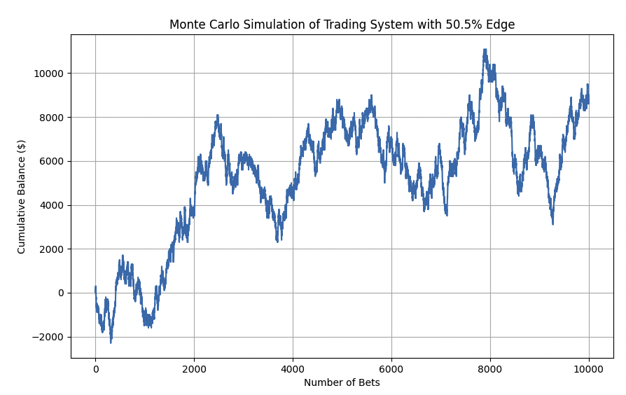
50.5% Edge

With a 50.5% edge, there were some initial losses (down about or close to $2,000 during two points within the first 1,500 trials), but got better as time went on.

This shows that this kind of edge is valuable, but still comes with a lot of volatility.

On average, you’re still squeezing out less than a $1 per trade after 10,000 trials and have a lot of variance.

This is winning but would be psychologically difficult for many traders.

This might be analogous to the house edge in blackjack with perfect basic strategy, if blackjack pays 3:2.

The casino will win over time with lots of hands and tables going, but players can have good luck in the short run – which can mean over 1,000-2,000 hands realistically during certain periods.

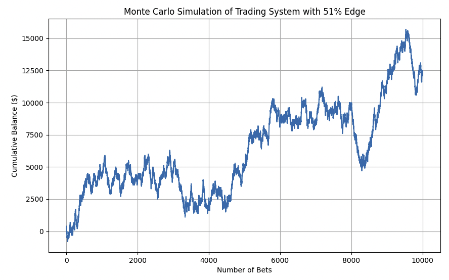
51% Edge

With a 51% edge, there may still be thousands of trials where you lose money.

For example, we were up right away in the early stages, but then plateaued or got worse until trial 5,000 or so before the next step up.

There was still a large drawdown after trial 8,000 before a strong winning streak showed the quality of this edge.

But still have to recognize there will be drawdowns and dry periods with a 51% edge.

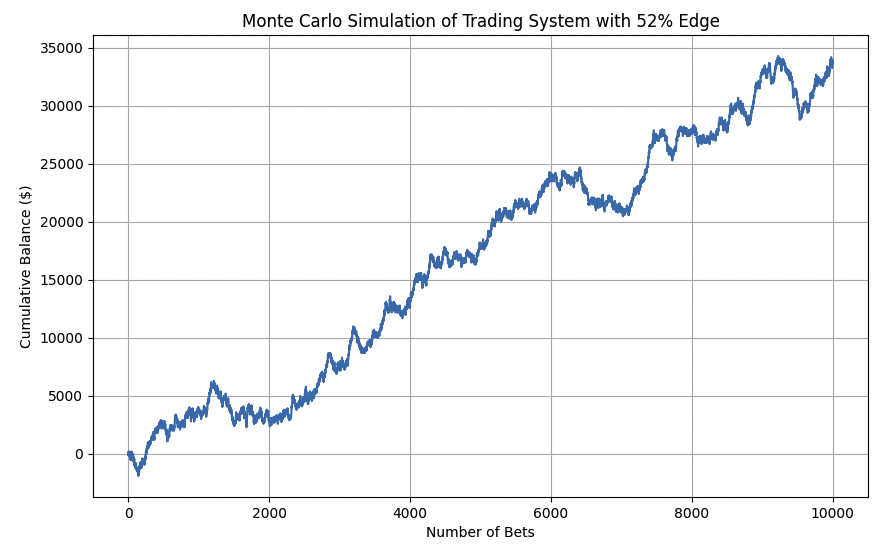
52% Edge

A 52% edge is where results start to get better.

At a 50.5% edge, we were early only around a $1 per trade in that simulation, but getting close to $3.50 per iteration here.

This might be analogous to

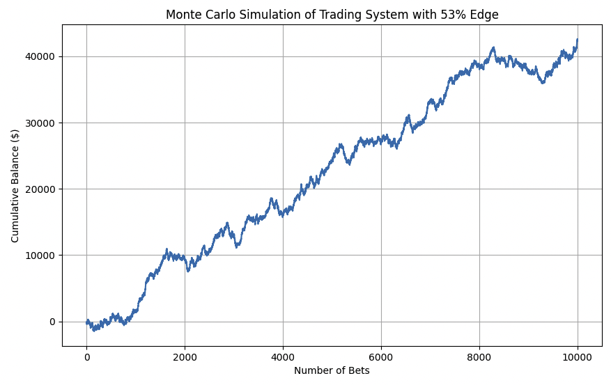
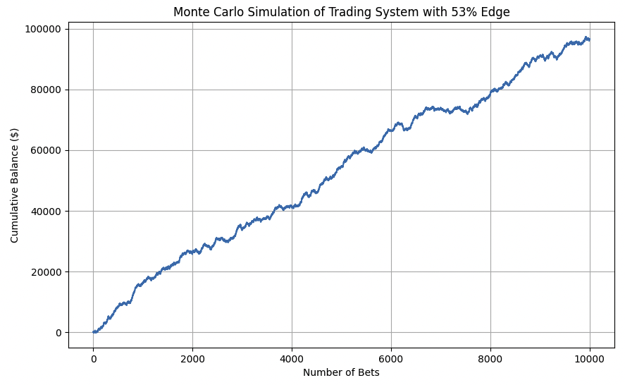
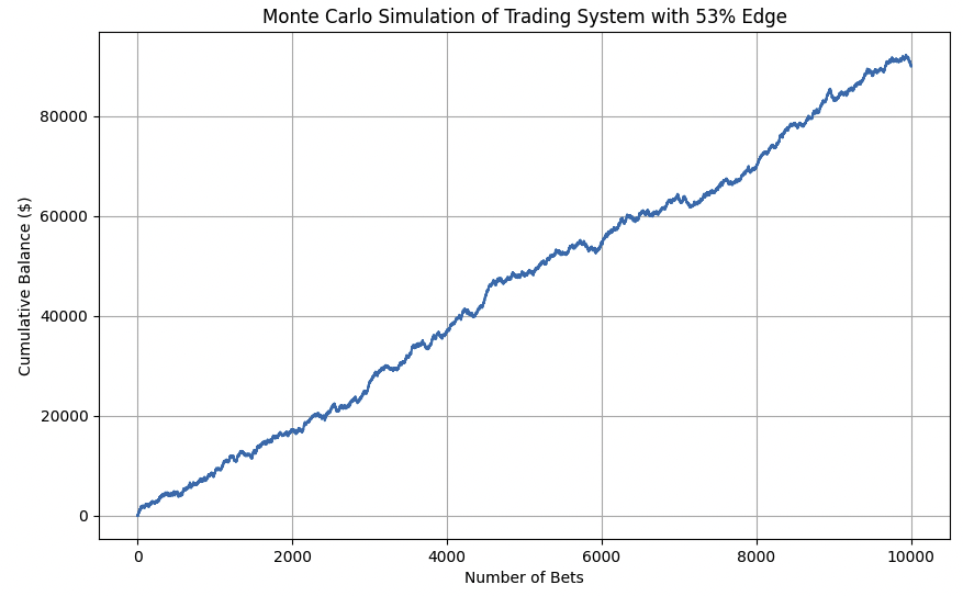
53% Edge

You can see at 53% with equal payout, skill becomes much more influential over variance.

54% Edge

As we get up to a 54% edge, the probability of a loss over 1,000 trials gets increasingly lower.

And over 10,000 trials profitability is a virtual certainty.

55% Edge

And we get up to 55%, the edge over so many trials is extremely strong that it becomes increasingly more linear.

Let’s look at the broader set of variables that go into how long to test a trading strategy.

1. Market Conditions

Diverse Market Phases

Make sure the system is tested across different market environments, such as bull markets, bear markets, sideways markets, high/low growth, high/low inflation, and periods of high and low volatility.

This helps understand the strategy’s robustness and adaptability.

Seasonality

If the market or the asset being traded is subject to seasonal effects, the testing period should cover multiple seasons to capture these variations.

2. Trading Frequency

Number of Trades

The more trades the system generates, the shorter the required testing period might be.

A high-frequency trading system can be tested over a shorter time frame, while a system with infrequent trades may need a longer period to generate enough data.

Signal Frequency

Systems that trade based on frequent signals (e.g., intraday strategies) may require less calendar time but still a significant number of trades to test.

Scalability

This goes off what we just mentioned, but the more trials of something you can test, the faster you can get to the long run and understand if you have something viable.

Impact of Market Noise

Higher-frequency trading systems are more likely to be influenced by market noise, which can skew results over short periods.

Testing over a sufficient number of trades helps to filter out noise and reveal the underlying performance of the strategy.

3. System Stability

Consistency of Results

Test the system long enough to observe whether its performance is consistent over time.

This helps in identifying whether the system’s profitability is stable or just due to temporarily favorable markets.

Drawdowns

A longer testing period may reveal the system’s behavior during significant drawdowns, which helps better understand its risk profile.

4. Statistical Significance

Sample Size

A sufficient number of trades are needed to make the results statistically significant.

For systems with fewer trades, a longer time frame may be required to achieve a statistically valid sample size.

Overall, the length of testing should be adequate to provide sufficient statistical power to detect the true performance of the trading system.

This reduces the likelihood of Type II errors (failing to detect a true effect) and makes sure that the system’s edge is not missed due to insufficient data.

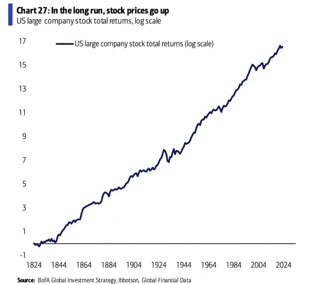
Over a long enough sample size, it starts to become clear whether a strategy is effective or not.

For example, stocks have been a good bet going back 200+ years.

Confidence Intervals

Testing should be long enough to provide a reasonable level of confidence that the system’s performance is not due to random chance.

This often involves calculating confidence intervals for the system’s returns.

Variability of Returns

Testing over a longer period allows for a better understanding of the variability in returns.

A sufficient sample size helps in accurately estimating the standard deviation of returns, which is important for understanding the risk associated with the trading system.

Distribution of Returns

If the system’s returns are assumed to follow a normal distribution, a larger sample size helps in validating this assumption.

Testing over a longer period helps understand the approximate distribution of returns, making statistical inferences more reliable.

Financial returns generally have fatter tails than what’s implied by the normal distribution, however.

5. Backtest Duration

Historical Data Availability

The availability of historical data can constrain the testing period.

More data allows for a longer and more comprehensive backtest.

Data Relevance

The chosen period should be relevant to current and expected future market environments.

For example, data from the 1980s may or may not be as relevant to today’s markets.

Stress Testing with Synthetic Data

• Forward Testing – Using synthetic data allows for forward testing under simulated extreme market conditions, helping to evaluate the system’s resilience.
• Diversifying Scenarios – Generating varied hypothetical scenarios, such as sudden market crashes or spikes in volatility. Helps in assessing how the system might perform when historical data is insufficient.
• Improving Robustness – Stress testing with synthetic data helps to understand that the trading strategy is not just optimized on or tailored to past markets but is robust enough to handle unforeseen future events.

6. Market Dynamics

Market Regimes

The system should be tested through different market regimes (e.g., pre- and post-financial crisis, low and high interest rate environments) to understand its performance across various economic environments.

Technology Changes

Technological advancements in trading (e.g., algorithmic trading) can change market behavior, so testing should cover periods before and after significant changes in market infrastructure.

7. Risk Management

Risk of Ruin

Test the system long enough to assess the probability of the system’s complete failure (risk of ruin), especially under extreme market conditions.

Drawdown Duration

Consider the maximum drawdown duration observed during testing to assess if the system can recover in a reasonable timeframe.

Position Sizing

Testing should include evaluating various position-sizing or betting strategies to determine how different bet sizes impact overall risk and potential drawdowns.

Proper position sizing helps in minimizing the risk of ruin and improving the system’s ability to endure adverse market environments.

Tail Risk

Evaluate the system’s performance in extreme scenarios, often referred to as tail risk.

Testing should account for rare but catastrophic events to ensure the strategy is prepared for extreme losses and doesn’t fail under unexpected conditions.

Risk-Adjusted Returns

Testing should also focus on calculating risk-adjusted performance metrics like the Sharpe and Sortino ratios.

These metrics provide a clearer picture of whether the returns are commensurate with the risk taken, ensuring that the strategy is not just profitable but also efficient in managing risk.

Think About Risk Holistically

Risk can mean many things.

There are volatility-based approaches, there’s tail risk, drawdowns, recovery period, skew, kurtosis, and many other things that risk can encapsulate.

8. Optimization vs. Overfitting

Out-of-Sample Testing

Be sure the system is tested on out-of-sample data (data not used in the development phase) to check for overfitting.

Longer testing periods can help identify if the system is genuinely robust or just overfitted to historical data.

Walk-Forward Analysis

Use walk-forward analysis to simulate real-time performance over different periods and reduce the risk of overfitting.

9. Real-World Constraints

Execution Costs

Consider slippage, commissions, and other transaction costs, which may vary over time.

Longer testing periods can reveal the impact of these costs more accurately.

Liquidity Constraints

The system should be tested over a period long enough to account for variations in market liquidity, which can affect trade execution and system performance.

Order Execution Speed

Test the system to assess how different market conditions affect order execution speed.

Delays in execution, especially in fast-moving markets, can impact profitability and risk, so it’s essential to evaluate this over varying time periods.

Market Impact

Larger trades may move the market, particularly in less liquid environments.

Testing should evaluate the impact of trade size on market prices and overall system performance, ensuring that the strategy remains viable when scaling up.

Bid-Ask Spread

The bid-ask spread can widen during volatile periods or low liquidity, increasing the cost of entering and exiting positions.

Testing over a range of conditions helps in understanding how fluctuating spreads affect net returns and whether the system can remain profitable under different spread scenarios.

10. Behavioral and Psychological Factors

The system should be tested long enough to so that it aligns with the trader’s psychological comfort.

If a system undergoes extended drawdowns or periods of underperformance, it might not be sustainable for a trader to follow it.

Overall

The appropriate duration for testing a trading system will vary depending on these factors.

In general, a longer testing period across varied market environments provides greater confidence in the system’s robustness and reliability.

For long-term trading strategies, it’s practical to conduct backtesting over years or decades. 

In contrast, shorter-term strategies with abundant data and frequent trades can often be tested effectively over a shorter period.