Reinforcement Learning Algorithms for Trading

A variety of reinforcement learning algorithms have been explored for trading applications.

Here, we look at key RL algorithms and how they apply to markets ranging from stocks and currencies to commodities and bonds.

Key Takeaways – Reinforcement Learning Algorithms for Trading

• RL algorithms help trading agents learn strategies that maximize returns by interacting with market data over time.
• Q-learning is foundational but struggles with complex, real-world markets.
• DQN scales Q-learning using deep networks to handle high-dimensional inputs.
• Policy Gradient methods optimize directly for trading goals like Sharpe ratio (or risk-adjusted returns more generally).
• Actor-Critic algorithms combine value and policy learning, great for continuous actions.
• TRPO is conceptually such that trading strategies change cautiously by enforcing stable updates. This avoids risky over-adjustments in more volatile markets.
• PPO is the top choice today—stable, efficient, and well-suited for portfolio management and trade execution.
• We explain how to build an RL algorithm at the end of the article.
  • Included is some basic code
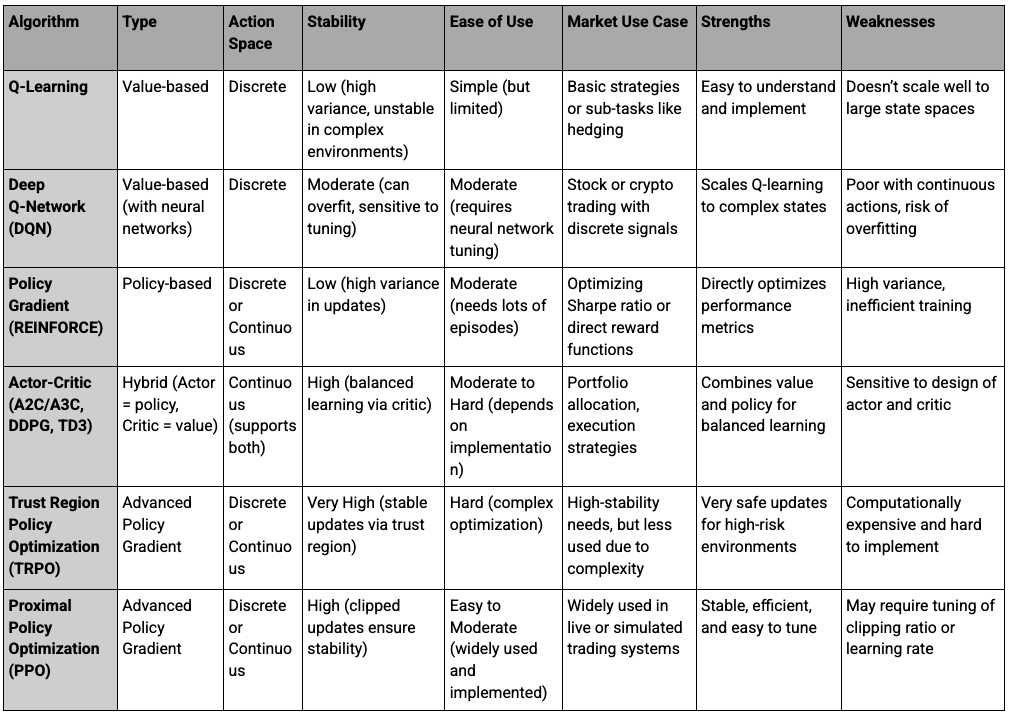
• We have a chart below for more comparisons of the various approaches:

Q-Learning and Its Applications in Trading

Q-learning is one of the simplest and earliest RL algorithms.

It’s a model-free method that learns what’s called a Q-value for each state-action pair – essentially, the expected reward of taking a certain action from a given state and following the optimal policy thereafter​.

In a trading scenario, a “state” could be a vector of recent market indicators (prices, technical signals, etc.), and an “action” could be something like buy, sell, or hold.

Q-learning iteratively updates its Q-values based on the reward received and the maximum expected future reward, using the Bellman equation.

Over time, the Q-values are supposed to converge such that the agent can choose the best action (highest Q-value) for each observed state.

In practice, vanilla Q-learning has limitations in trading because financial state spaces are huge and continuous (prices can take many values, indicators are continuous, etc.).

Traditional Q-learning stores a Q-table (state-action lookup table), which is not feasible for the complexity of real markets.

Early academic applications of Q-learning in finance therefore often simplified the problem – for example, discretizing states into bins (e.g., market going up, down, or flat) and actions into coarse categories, or applying Q-learning to smaller sub-problems like trading a single asset with a few discrete signals.

One notable use case was in option hedging: researchers applied a form of Q-learning to learn hedging strategies.

Modeling an options environment and using Q-learning, they found the algorithm could efficiently learn a hedging policy that managed risk as well as or better than traditional techniques, even when considering transaction costs.

Basic Q-learning by itself is rarely used for full-scale trading systems today. But it’s conceptually important – many advanced methods build on the idea of learning value functions.

Moreover, Q-learning can work in trading when combined with function approximation (as we’ll see with DQN below) or when tackling specific simplified tasks.

It laid the groundwork for thinking about trading in an RL framework, where the goal is to learn the value of actions (trades) and thereby derive an optimal strategy.

Deep Q-Networks (DQN) and Their Role in Market Prediction

Deep Q-Networks (DQN) revolutionized reinforcement learning by allowing Q-learning to scale to complex, high-dimensional problems (like markets).

A DQN uses a neural network to approximate the Q-value function, instead of a literal table. This was famously applied by DeepMind to play Atari games, and the same idea has been applied to trading.

In a trading DQN, the neural network takes as input the state (which could be a window of recent prices, technical indicators, etc.) and outputs Q-values for each possible action (e.g., buy, sell, hold).

The agent then selects actions according to these Q-value estimates, and the network is trained with experience replay and temporal-difference updates to minimize the error in the Q-value predictions.

DQN’s ability to handle continuous state spaces and find patterns is a major advantage for trading.

For example, a DQN can learn to predict or rather estimate the long-term value of buying or selling in particular market conditions/environments.

If the network architecture is sufficiently deep, it can capture nonlinear relationships in the data – for instance, recognizing a combination of rising momentum and low volatility as a particularly good buying opportunity (just as an illustrative example).

There have been numerous projects and studies where DQN agents were trained on stock market data. Many report that the DQN-based agents could indeed learn profitable trading policies or at least beat naive benchmarks in simulation​.

One study demonstrated the application of Deep Reinforcement Learning (DRL) to cryptocurrency trading, looking at how hierarchical problem decomposition, model-based RL, risk measures, and state representations can improve DRL trading agents. But here they found that even state-of-the-art DRL agents can struggle with market noise, overfitting, and unstable performance across different assets.

DQN Limitations

A key limitation is that DQN (and Q-learning in general) traditionally handles discrete actions.

In many trading scenarios, actions can be continuous (e.g., adjust portfolio weights by some percentage, or trade 0.5 lots of currency).

Discretizing actions (like “buy 100 shares” as one action) can limit the strategy’s flexibility.

Moreover, training deep networks that don’t overfit is tricky – a DQN might latch onto spurious correlations in historical data.

Researchers often incorporate techniques like dropout, early stopping, or ensemble methods to make DQN strategies stronger.

DQN Uses Are Growing

Nonetheless, DQN and its variants (Double DQN, Dueling DQN, etc.) remain popular for trading problems where the action space is reasonably discrete.

They serve as a bridge between simple value-based methods and more complex policy-based methods, by using deep learning to approximate the value function.

The success of DQN in other fields has certainly inspired many financial engineers to try it on market prediction and trading tasks, and it continues to be an area of active experimentation in the trading community (with open-source implementations available that traders tinker with for their own strategies).

Policy Gradient Methods and Their Effectiveness in Trading Strategies

Policy gradient (PG) methods take a different approach from value-based methods like Q-learning.

Instead of learning “value of actions,” a policy gradient method directly learns a parameterized policy that maps states to a probability distribution over actions.

The algorithm then adjusts the policy parameters in the direction that increases expected reward (hence “policy gradient”)​.

The quintessential example is the REINFORCE algorithm (also called Monte Carlo policy gradient), which adjusts the policy parameters based on episodes of experience, weighting actions by the returns that followed them.

In trading, policy gradient methods can be appealing for several reasons:

They can naturally handle continuous action spaces

For example, an agent could have a policy that outputs a continuous number representing, say, the proportion of the portfolio to allocate to stocks vs. bonds.

This is difficult for a pure DQN (which would require discretization), but straightforward for a policy network that outputs, say, a Gaussian distribution for an action.

They allow optimizing arbitrary reward objectives

In trading, we often care about metrics like the Sharpe ratio (a popular type of risk-adjusted return) or drawdown in addition to raw profit.

It’s possible to design the reward function to reflect these (though with caution), and policy gradient methods will directly attempt to optimize that reward.

A famous early example was Recurrent Reinforcement Learning (RRL) by Moody and Saffell (1999-2001), which is effectively a policy gradient method that directly maximized a risk-adjusted return (specifically, differential Sharpe ratio) for trading​.

They found this direct approach produced better trading strategies than indirect methods like Q-learning, in part because it could incorporate risk-adjusted rewards and didn’t need to estimate value for every state​.

In their work, RRL was used to discover trading policies that outperformed benchmarks, including an application to currency trading and asset allocation.

Policy gradient methods can be simpler to integrate with existing strategy frameworks

For instance, if a hedge fund already has a parametric trading strategy (like “buy when score S > 0.5, sell when S < -0.5, with some thresholds to tune”), one could interpret that as a policy and use policy gradient methods to fine-tune those parameters to maximize returns.

However, pure policy gradient methods like REINFORCE have high variance in gradient estimates, which can make training unstable or slow.

They require a lot of training episodes to get right. In trading, generating many independent episodes is a challenge (we can’t truly reset the market and run it forward many times).

This is one reason why actor-critic methods (discussed next) are often favored – they reduce variance by using a critic (value function) alongside the policy.

Summary

Policy gradient methods enable direct optimization of trading performance metrics.

They’ve been effective in various research settings – for example, strategies that explicitly maximize the Sharpe ratio or minimize volatility can be encoded via policy gradients.

The flexibility in defining the goal (reward) is a major edge.

As long as one can simulate or sample trading trajectories, policy gradients will try to improve the policy toward the desired outcome.

Many modern algorithms (PPO, TD3, etc.) are essentially enhanced policy gradient methods at their core.

Actor-Critic Methods for Balancing Exploration and Exploitation

Actor-Critic algorithms combine the best of both worlds from value-based and policy-based approaches.

In this framework, there is an Actor (which proposes actions according to a policy, like a policy network) and a Critic (which evaluates how good the action was in terms of future reward, often by estimating a value function).

The critic helps guide the learning of the actor by critiquing its actions, which significantly reduces the variance of policy gradient updates.

Common examples of actor-critic algorithms include Advantage Actor-Critic (A2C/A3C), Deep Deterministic Policy Gradient (DDPG), and others like TD3.

Continuous Action Spaces

In trading, actor-critic methods have gained popularity because they can handle continuous action spaces and complex policies while training more stably than pure policy gradient.

The critic (value estimator) provides a baseline that makes the reward feedback less noisy.

For instance, instead of just telling the policy “you made $X profit by the end of the episode” (which could be high variance), the critic can learn at each time step, “given the state, your action was better or worse than expected.”

This granular feedback is very useful in volatile financial environments.

Exploration vs. Exploitation

Actor-critic methods are useful for balancing exploration and exploitation.

The actor will try actions according to its policy (which, especially early in training, might be exploratory), and the critic quickly learns to evaluate those.

If an action was poor, the critic’s value estimate for that state-action will be low, which in turn adjusts the actor to reduce the probability of that action in the future.

Conversely, if an action yielded unexpectedly good results, the critic’s valuation goes up and the actor learns to favor that action.

This mechanism ensures that the agent can explore new strategies but get guided feedback to exploit the ones that show promise.

Example

A concrete application example: consider an actor-critic RL model applied to a portfolio trading scenario with multiple assets (stocks, bonds, gold).

The actor could output an allocation (percentage weights to each asset) or trading signals for each asset, and the critic would estimate the expected portfolio return (or some utility) given the current market state and the proposed allocation.

Such a system was used in a study that trained specialized trading agents for different markets – an actor-critic neural network was used to manage trades in assets like Euro (currency), gold, and crude oil, and it achieved more efficient trading with reduced losses​.

The actor-critic agent in that case was able to adjust to different time periods and market environments, and notably minimized capital losses in volatile markets (gold and oil can be quite volatile) compared to baseline strategies​.

This highlights how actor-critic methods can incorporate risk management directly into the learning objective (the critic can be set to emphasize avoiding large losses, for instance).

Common Actor-Critic Algorithms

Common actor-critic algorithms in trading include:

• A3C/A2C, which have been used for trading single assets with continuous position sizes;
• DDPG (Deep Deterministic Policy Gradient), which is suitable for continuous action like setting buy/sell volume (it’s been applied to problems like optimal trade execution or portfolio allocation); and
• Twin Delayed DDPG (TD3), which addresses some DDPG pitfalls and has been used in trading simulations to stabilize learning of trading policies.

Overall, actor-critic frameworks are currently a workhorse for many DRL trading systems because of their balance of stability and flexibility.

They continue to be an area of active research – for example, combining actor-critic with attention mechanisms to focus on relevant market features, or multi-actor multi-critic systems for multi-asset portfolios.

Proximal Policy Optimization (PPO) and Trust Region Policy Optimization (TRPO)

Trust Region Policy Optimization (TRPO) and Proximal Policy Optimization (PPO) are advanced policy gradient methods that have proven effective, including in trading applications.

They were developed to address the instability of naive policy gradient methods by preventing the policy from changing too much in a single update (which can catastrophically degrade performance).

TRPO

Trust Region Policy Optimization (2015) gives stable policy updates by enforcing a constraint (approximately via KL-divergence) – i.e., that the new policy after an update is not too far from the old policy.

This “trust region” approach yielded very reliable improvements in control tasks and games.

In trading, one can see the appeal: you don’t want your trading strategy to shift wildly from one training iteration to the next, as that could cause erratic behavior (e.g., suddenly going from cautious to all-in risk).

TRPO would guard against such swings. But TRPO is computationally heavy and complex to implement, as it involves solving a constrained optimization problem each step.

This can be a drawback in finance where one might want to retrain frequently or on large datasets.

In fact, in practice TRPO’s complexity has made it less popular for financial market use; researchers found it cumbersome and often unnecessary when PPO was introduced as a simpler alternative​.

PPO

Proximal Policy Optimization (2017) was introduced as a simpler, more computationally efficient cousin of TRPO that still achieves the goal of bounded policy updates.

PPO uses a clipping mechanism in the objective function to discourage the new policy from deviating too far from the old one.

In essence, if the policy tries to change an action probability by more than (say) 20% at once, the clipping term penalizes that update.

PPO has become very popular due to its ease of implementation and quality performance.

In financial trading contexts, PPO is often the go-to algorithm for many because it reliably learns good policies without the need for delicate tuning of constraints.

TRPO vs. PPO

Here’s a table comparing TRPO and PPO.

Why are PPO (and TRPO) well-suited for trading?

One reason is the stability of learning.

Financial markets can be unforgiving of a “bad policy” – if during training the agent suddenly does something very risky (exploiting a perceived short-term gain), it might incur a huge loss that skews training or even worse – e.g., bankrupts a trading account in simulation.

PPO’s clipped updates reduce this risk by making incremental improvements.

It strikes a balance between exploration (trying new strategies) and exploitation (refining what works), without overshooting​.

This balanced approach means the RL agent is less likely to overfit to random noise or to take extreme, out-of-distribution actions.

As one analysis noted, PPO helps make sure the model doesn’t overfit to market noise or make extreme trades, providing a framework for developing trading strategies​.

Another advantage: PPO (and TRPO) work seamlessly with actor-critic frameworks. Hence, they can handle continuous actions effectively.

PPO is useful for cases like deciding continuous position sizes or portfolio weights.

For example, adjusting a portfolio allocation by small increments can be naturally modeled with PPO.

In contrast, simpler algorithms like DQN are better suited for discrete actions (e.g., a yes/no trading decision)​.

So for complex decisions – imagine an algorithm that needs to dynamically rebalance a portfolio among stocks, bonds, currencies, etc. – PPO can manage that where something like DQN would struggle.

In practice, PPO has been used in various trading simulations and research.

Some applications include optimal trade execution (where the action is how much of an order to execute now vs later), portfolio optimization, and even high-frequency trading strategy design.

Because of its efficiency, PPO allows frequent policy updates which is key for fast-moving markets​  – an agent can learn on the fly or adapt daily without requiring enormous batch runs.

To illustrate, a study on portfolio management using PPO found that it could learn to allocate assets in a way that outperformed traditional mean-variance solutions, thanks to being able to continuously adjust in response to market changes​.

For example, a strategy involving pairs trading optimization could use PPO to decide when to long/short a pair of stocks, leveraging PPO’s stability to get consistent performance.

TRPO paved the way for safer policy updates, and PPO made it practical.

PPO has essentially become a standard tool in the arsenal for RL-based trading, given its efficiency, stability, and flexibility​.

Many cutting-edge trading AI implementations use PPO or similar clipped policy gradient methods under the hood, often tuned to maximize a specific objective (like Sharpe ratio, downside protection, etc.) while keeping the policy updates reliable.

How to Build an RL Algorithm Step-by-Step

Step 1: Define the Environment

Choose a market environment (e.g., stock, ETF, crypto, etc.).

At each time step, the environment provides:

• State = recent price data, indicators, etc.
• Reward = profit/loss or custom metric (e.g., Sharpe ratio).
• Actions = Buy, Sell, or Hold (or portfolio weights if continuous).

Step 2: Choose the Algorithm

Start simple:

• Q-learning for discrete actions.
• DQN if using price history or indicators with neural networks.
• PPO or Actor-Critic for continuous or complex actions.

Step 3: Build the Agent

• For Q-learning = use a Q-table or a neural network.
• For DQN/PPO = use a neural net to predict action-values or policies.

Structure input to include price history, indicators, or portfolio context.

Step 4: Training Loop

1. Initialize agent and environment.
2. For each episode:
   • Reset environment
   • Loop through each time step:
     • Get current state
     • Choose action (based on current policy or Q-values)
     • Step the environment → get next state, reward
     • Store experience (state, action, reward, next state)
     • Update model with batch of experiences
3. Repeat for many episodes to improve.

Step 5: Evaluation

After training, test the agent on unseen market data.

Measure performance with:

• Cumulative return
• Sharpe ratio
• Drawdown
• Hit rate

Optional

Add stop-loss rules, transaction costs, or risk controls to make it more realistic.

Example Code

Below is basic Python code for a simple Q-learning agent for trading — applied to a toy environment where the agent can choose to Buy, Sell, or Hold based on simplified price movements.

This is just a starting point to help you understand the RL structure. You can upgrade this later to DQN or PPO.

pip install numpy pandas

import numpy as np

import pandas as pd




# Sim the price data

prices = np.random.normal(loc=0.0, scale=1.0, size=1000).cumsum()

price_df = pd.DataFrame({'price': prices})




# Now define your states and actions

states = ['up', 'down', 'flat']

actions = ['buy', 'sell', 'hold']

q_table = pd.DataFrame(0, index=states, columns=actions)




# Hyperparameters

alpha = 0.1      # this is the learning rate

gamma = 0.9      # discount factor

epsilon = 0.1    # exploration rate




# Define your state from the price change

def get_state(change):

    if change > 0.5:

        return 'up'

    elif change < -0.5:

        return 'down'

    else:

        return 'flat'




# Training loop

position = 0  # +1 if holding stock, 0 otherwise

for t in range(1, len(prices) - 1):

    price_change = prices[t] - prices[t - 1]

    state = get_state(price_change)




    if np.random.rand() < epsilon:

        action = np.random.choice(actions)

    else:

        action = q_table.loc[state].idxmax()




    # Reward function (simple)

    reward = 0

    if action == 'buy':

        position = prices[t]

    elif action == 'sell' and position:

        reward = prices[t] - position

        position = 0




    # Get next state

    next_price_change = prices[t + 1] - prices[t]

    next_state = get_state(next_price_change)




    # Q-value update

    old_value = q_table.loc[state, action]

    future_max = q_table.loc[next_state].max()

    q_table.loc[state, action] = old_value + alpha * (reward + gamma * future_max - old_value)




# Show the learned policy

print("Learned Q-Table:")

print(q_table)

What This Does

• Simulates a random walk market.
• Categorizes market into simple states (up, down, flat).
• Learns whether to buy, sell, or hold depending on recent price changes.
• Stores and updates action values in a Q-table.

This is deliberately basic for clarity.

You can later:

• Replace random walk with real historical price data.
• Use more features (e.g., RSI, moving averages for those using traditional technical indicators).
• Upgrade to DQN with PyTorch or TensorFlow for deep learning.

Results

Running the code, you get something like:

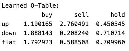
The Learned Q-Table represents the expected rewards for taking each action (buy, sell, hold) in different market states (up, down, flat), based on the reinforcement learning agent’s experience.

How to Read It

Each number is a Q-value, meaning how much reward the agent expects from that action in that state.

Example Interpretation:

• When the market is UP (up row):
  • buy: 1.19 → The agent expects a moderate gain if it buys.
  • sell: 2.76 → The agent expects a higher gain if it sells.
  • hold: 0.45 → The agent expects a low reward if it holds.
  • Best Action: Sell, because 2.76 is the highest.

• When the market is DOWN (down row):
  • buy: 1.88 → The agent thinks buying might be profitable.
  • sell: 0.21 → The agent expects a loss if it sells.
  • hold: 0.71 → Holding is better than selling but worse than buying.
  • Best Action: Buy, because 1.88 is the highest.

• When the market is FLAT (flat row):
  • buy: 1.79 → The agent expects decent gains if it buys.
  • sell: 0.59 → Selling isn’t great here.
  • hold: 0.71 → Holding is better than selling but worse than buying.
  • Best Action: Buy, because 1.79 is the highest.

Final Takeaway

• The Q-table shows what the agent has learned about which actions are best in different market conditions.
• In this case, the agent learned to sell in up markets, buy in down markets, and buy in flat markets.

This strategy makes sense in many cases but should be tested on real data.