Volatility Surface (Concept & Trade Examples)


A volatility surface is a three-dimensional representation of option implied volatilities across different strike prices and expiration dates.
It’s an important form of visual analysis in options pricing and risk management.
It provides a view of how the market perceives volatility for a particular underlying asset.
Key Takeaways – Volatility Surface
- Shape reveals market sentiment – A steep skew indicates heightened downside risk, while a flatter surface suggests more balanced expectations.
- Term structure matters – Longer-dated options with higher implied volatility can signal sustained market uncertainty (i.e., wider implied probability distributions than normal).
- Surface dynamics predict market moves – Sudden changes in the surface, especially in specific areas, often precede significant price movements in the underlying asset.
- Example Trades – We give example trades later in the article that use information taken from volatility surfaces to put on certain trades.
The Concept of Implied Volatility
Before going into volatility surfaces, it’s important to understand implied volatility.
This is the market’s forecast of a likely movement in a security’s price, derived from option prices rather than historical price data.
Implied volatility is a critical component in options pricing models, such as the Black-Scholes model.
From Volatility Smile to Surface
The volatility surface evolved from the concept of the volatility smile, which plots implied volatility against strike prices for a single expiration date.
This gives a 2D visual.
The surface extends this idea to include multiple expiration dates, creating a three-dimensional representation, which we’ll cover below.
Components of a Volatility Surface
A volatility surface consists of three main components:
- Strike Price (X-axis)
- Time to Expiration (Y-axis)
- Implied Volatility (Z-axis)
Strike Price
The strike price, or exercise price, is the price at which an option contract can be exercised.
It forms one dimension of the volatility surface, allowing traders to visualize how implied volatility changes across different strike prices.
Time to Expiration
The time to expiration, also known as maturity or tenor, represents the time remaining until the option contract expires.
This forms the second dimension of the volatility surface and enables the observation of term structure in implied volatilities.
Implied Volatility
Implied volatility forms the third dimension of the surface.
This represents the market’s expectation of future volatility for the underlying asset.
It’s derived from option prices using an options pricing model, typically the Black-Scholes model (though many others are viable).
Constructing a Volatility Surface
Building a volatility surface involves several steps and considerations:
Data Collection
The first step is gathering option price data for various strike prices and expiration dates.
This data is typically obtained from market sources or option pricing feeds.
Implied Volatility Calculation
Using the collected price data, implied volatilities are calculated for each option using an option pricing model.
This process often involves numerical methods, as most pricing models don’t have a closed-form solution for implied volatility.
Interpolation and Extrapolation
Since market data may not be available for all possible combinations of strike prices and expiration dates, interpolation and extrapolation techniques are used to fill in the gaps.
Common methods include:
- Cubic spline interpolation
- SABR (Stochastic Alpha Beta Rho) model
- Local volatility models
Smoothing Techniques
To reduce noise and irregularities in the surface, various smoothing techniques may be applied.
These help in creating a more stable and realistic representation of market expectations.
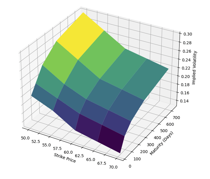
Volatility Surface Modeled with Code
We can design a diagram of a volatility surface by designing some arrays and then plotting them:
import numpy as np

import matplotlib.pyplot as plt

from mpl_toolkits.mplot3d import Axes3D

# Sample data for a 3D volatility term structure

strikes = np.array([50, 55, 60, 65, 70])

maturities = np.array([30, 90, 180, 365, 730])

implied_vols = np.array([

[0.20, 0.18, 0.15, 0.14, 0.13],

[0.22, 0.20, 0.18, 0.17, 0.16],

[0.25, 0.22, 0.20, 0.19, 0.18],

[0.28, 0.25, 0.22, 0.21, 0.20],

[0.30, 0.27, 0.24, 0.23, 0.22]

])

# Meshgrid for plotting

X, Y = np.meshgrid(strikes, maturities)

Z = implied_vols

# Plot the 3D volatility term structure

fig = plt.figure(figsize=(12, 8))

ax = fig.add_subplot(111, projection='3d')

ax.plot_surface(X, Y, Z, cmap='viridis')

ax.set_title('3D Volatility Term Structure')

ax.set_xlabel('Strike Price')

ax.set_ylabel('Maturity (Days)')

ax.set_zlabel('Implied Volatility')

plt.show()
3D Volatility Surface
Characteristics of Volatility Surfaces
Volatility surfaces exhibit several notable characteristics:
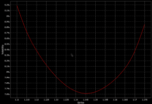
Volatility Smile
The volatility smile is a cross-section of the surface for a single expiration date.
It typically shows higher implied volatilities for both in-the-money and out-of-the-money options compared to at-the-money options.
Term Structure
The term structure of volatility refers to how implied volatility changes with time to expiration.
It can be observed by examining a cross-section of the surface for a fixed strike price.
Skew
Volatility skew refers to the asymmetry in implied volatilities across strike prices.
A negative skew, common in equity markets, shows higher implied volatilities for lower strike prices.
Surface Dynamics
Volatility surfaces are not static; they evolve over time as markets change.
Now let’s get into examples.
These examples will illustrate how traders can use the information contained in volatility surfaces to inform their trading decisions.
Be sure to understand and stress test these strategies further if you consider putting them on in live trading with real money.
1. Volatility Skew Trade: Put Spread
Trade Structure
- Sell an out-of-the-money (OTM) put option
- Buy a further OTM put option with the same expiration
Reasoning
Volatility skew typically shows higher implied volatilities for OTM puts compared to at-the-money (ATM) options.
This is often referred to as the “volatility smile” or “skew.”
Traders can potentially profit from this by selling overpriced OTM puts and buying cheaper, further OTM puts as protection.
The trade looks to take advantage of the steepness of the volatility skew while limiting downside risk.
If the skew flattens (i.e., the difference in implied volatility between the two strike prices decreases), the trade can be profitable even if the underlying asset doesn’t move a lot.
Example Scenario
Let’s say a stock is trading at $100, and the 90-strike put has an implied volatility of 30%, while the 80-strike put has an implied volatility of 35%.
A trader might:
- Sell the 90-strike put
- Buy the 80-strike put
If the skew flattens, perhaps with the 90-strike implied volatility rising to 32% and the 80-strike falling to 33%, the spread will narrow.
Also note that higher implied volatility at a strike doesn’t mean it’s a more expensive option in dollar terms, just more expensive in implied volatility terms.
2. Calendar Spread: Exploiting Term Structure and Theta Decay
Trade Structure
- Sell a near-term ATM option
- Buy a longer-term ATM option of the same type (call or put)
Reasoning
The volatility surface often shows a term structure where longer-dated options have higher implied volatilities than shorter-dated ones.
This is because there’s more uncertainty over longer time horizons.
Traders can potentially profit from this by selling shorter-term options (which decay faster) and buying longer-term options.
If implied volatilities remain stable or increase, the longer-term option may gain value faster than the shorter-term option loses value.
Example Scenario
Consider a stock trading at $100.
The 1-month ATM call might have an implied volatility of 20%, while the 3-month ATM call has an implied volatility of 25%.
A trader could:
- Sell the 1-month 100-strike call
- Buy the 3-month 100-strike call
If overall market volatility increases, the longer-term option is likely to appreciate more than the shorter-term option.
3. Butterfly Spread: Exploiting Volatility Smile
Trade Structure
- Buy one ATM option
- Sell two OTM options equidistant from the ATM strike
- Buy one further OTM option at twice the distance
Reasoning
The volatility smile often shows higher implied volatilities for both ITM and OTM options compared to ATM options.
A butterfly spread can potentially profit from this pattern by buying the relatively cheaper ATM option and selling the more expensive OTM options.
This trade benefits if the underlying asset remains stable and if the volatility smile flattens (i.e., if the difference in implied volatilities between ATM and OTM options decreases).
Example Scenario
For a stock trading at $100:
- Buy one 100-strike call
- Sell two 110-strike calls
- Buy one 120-strike call
If the stock price remains close to $100 and the volatility smile flattens, the ATM option may retain more value while the OTM options lose value.
4. Volatility Dispersion Trade
Trade Structure
- Sell options on an index
- Buy options on individual components of the index
Reasoning
The volatility surface of an index often differs from the surfaces of its component stocks.
Index options might be priced with lower implied volatilities due to diversification effects.
This can create opportunities for traders to sell “expensive” single-stock options and buy “cheap” index options.
This trade can be profitable if the implied volatilities of individual stocks decrease more (or increase less) than the index implied volatility.
Example Scenario
Consider a tech-focused index and its top components. A trader might:
- Sell ATM calls on Apple, Microsoft, and Google
- Buy ATM calls on the tech index
If the individual stock volatilities decrease while the index volatility remains stable, this trade could be profitable.
Special Risks & Considerations
With this, not all stocks within an index will have liquid individual options – or options at the timeframe you want to trade.
The fortunate news is that for market cap-weighted indexes like the S&P 500, the largest stocks tend to take up a large bulk of the index and be the most liquid (in terms of the stock and options).
This can help create the single-stock portion of the trade that approximates the index fairly quickly.
5. Volatility Cone Trade
Trade Structure
- Buy options when implied volatility is near the bottom of its historical range
- Sell options when implied volatility is near the top of its historical range
Reasoning
A volatility cone shows the range of implied volatilities for different time horizons based on historical data.
Traders can use this to identify when current implied volatilities are unusually high or low compared to historical norms.
This strategy assumes mean reversion in volatility – that is, extremely high or low volatilities tend to move back toward average levels over time.
Example Scenario
If the 30-day implied volatility for a stock is currently 15%, but the volatility cone shows that it has historically ranged between 20% and 30% for this time horizon, a trader might:
- Buy 30-day ATM options, expecting implied volatility (and thus option prices) to increase
Conversely, if the current 30-day implied volatility is 35%, above the historical range, the trader might sell options, expecting implied volatility to decrease.
6. Cross-Asset Volatility Arbitrage
Trade Structure
- Identify assets with historically correlated volatilities
- Buy options on the asset with relatively low implied volatility
- Sell options on the asset with relatively high implied volatility
Reasoning
Different assets, especially those in related sectors or with similar risk profiles, often have correlated volatilities.
When their implied volatilities diverge significantly from historical norms, it may present a trading opportunity.
This strategy assumes that the volatilities will converge back to their historical relationship.
Example Scenario
Consider two major oil companies that historically have had similar implied volatilities.
If Company A’s 3-month ATM options suddenly have much higher implied volatility than Company B’s, a trader could consider:
- Selling Company A’s 3-month ATM options
- Buying Company B’s 3-month ATM options
If the volatilities converge, this trade could be profitable.
Other Considerations
Volatility surfaces often exhibit interconnected behaviors across asset classes.
For example, equity volatility spikes might correlate with bond yield curve shifts.
Understanding these relationships can help with portfolio management and overall risk assessment.
7. Volatility Surface Momentum Trade
Trade Structure
- Identify consistent changes in the shape of the volatility surface over time
- Take positions that benefit from the continuation of this trend
Reasoning
Volatility surfaces can exhibit momentum effects, where changes in the surface shape tend to continue in the same direction for some time.
This could be due to persistent market sentiment or ongoing market events.
Traders can potentially profit by identifying these trends and positioning themselves to benefit if they continue.
Example Scenario
If a trader notices that the short-term implied volatilities for a stock have been consistently increasing relative to long-term implied volatilities over the past few weeks, they might:
- Sell longer-dated options
- Buy shorter-dated options
This trade would benefit if the trend of increasing short-term volatilities continues.
Summary of Trade Examples
These example trades show how the information contained in volatility surfaces can be used to inform trading decisions.
Each trade attempts to capitalize on specific characteristics or dynamics of the volatility surface:
- The Volatility Skew Trade exploits the tendency for OTM options to have higher implied volatilities.
- The Calendar Spread takes advantage of the term structure of volatility.
- The Butterfly Spread profits from the shape of the volatility smile.
- The Volatility Dispersion Trade leverages differences between index and component volatilities.
- The Volatility Cone Trade uses historical volatility ranges to identify potential mean reversion opportunities.
- The Cross-Asset Volatility Arbitrage looks for discrepancies in implied volatilities between related assets.
- The Volatility Surface Momentum Trade attempts to profit from ongoing trends in surface shape changes.
Of course, these trades also carry risks.
Changes in the underlying asset price, shifts in market sentiment, and other factors can affect the volatility surface in unexpected ways.
Also, these trades often involve multiple options, which can result in complex risk profiles that make them hard to manage.
Successfully putting on these strategies requires not only a deep understanding of options and volatility dynamics but also sophisticated modeling techniques, access to quality data, and strong risk management practices.
Moreover, as these strategies become more widely known and implemented, their profitability may decrease.
The market’s efficiency tends to erode edges over time.
This requires traders to continually innovate and find new ways to extract value from the information contained in volatility surfaces.
This gets into advanced concepts like higher-order moments of volatility surfaces that no only explore the skew in volatility or its kurtosis (the thickness of the tail), but 5th, 6th, and nth-order moments that go deeper into the tailedness of the volatility surface.
Applications of Volatility Surfaces
Volatility surfaces have numerous applications in finance:
Option Pricing
The surface provides a framework for pricing options more accurately, especially for exotic options that depend on the entire volatility structure.
Risk Management
Traders and risk managers use volatility surfaces to assess and manage portfolio risk – particularly for positions with exposure to volatility.
Volatility Trading
Volatility surfaces enable traders to identify and exploit opportunities in the volatility market.
Examples include relative value trades or volatility arbitrage.
Model Calibration
Quants use volatility surfaces to calibrate more advanced option pricing models, so that they accurately reflect market prices.
Challenges in Working with Volatility Surfaces
Despite their usefulness, volatility surfaces present several challenges:
Data Quality and Availability
Constructing accurate surfaces requires high-quality market data, which may not always be available – especially for less liquid options.
Model Risk
The choice of interpolation and extrapolation methods can significantly impact the surface’s shape, introducing model risk.
Computational Complexity
Building and maintaining volatility surfaces, especially in real-time, can be computationally intensive.
Interpretation
Interpreting the information contained in a volatility surface requires expertise and can be challenging, especially when surfaces exhibit complex shapes or dynamics.
Advanced Topics in Volatility Surfaces
Several advanced topics are associated with volatility surfaces:
Local Volatility Models
Local volatility models attempt to create a deterministic volatility function that perfectly fits the observed volatility surface.
Stochastic Volatility Models
Models like Heston’s stochastic volatility model try to capture the dynamics of the volatility surface by introducing a stochastic process for volatility itself.
Volatility Surface Arbitrage
Sophisticated traders look for arbitrage opportunities across the volatility surface.
They look to exploit inconsistencies in option prices or implied volatilities.
Machine Learning Approaches
Recent focus has explored the use of machine learning techniques, such as neural networks, to model and predict volatility surfaces.
Deep learning models can capture complex patterns and non-linear relationships, potentially improving prediction accuracy.
Big data analysis allows for real-time processing of vast amounts of market information.
This can enable more dynamic and responsive surface modeling.
Statistical Moments of Volatility Surfaces
Statistical moments of volatility surfaces help understand the distribution and characteristics of implied volatilities across strike prices and expiration dates.
The mean represents the average level of implied volatility, offering a general sense of market uncertainty.
- Variance measures the dispersion of volatilities, indicating the range of market expectations.
- Skewness captures the asymmetry of the surface, with negative skew often indicating greater perceived downside risk.
- Kurtosis describes the “tailedness” of the distribution, with high kurtosis suggesting a higher probability of extreme events.
The 5th and 6th order moments, while less commonly used, can provide additional nuance.
The 5th moment (hyper-skewness) offers insights into the direction of extreme events, while the 6th moment (hyper-kurtosis) can indicate the likelihood of even more extreme events than captured by standard kurtosis.
These higher-order moments are useful for analyzing complex option strategies and managing tail risk in volatile markets.
They offer a more nuanced understanding of the “tailedness” and extreme event probabilities embedded in the volatility surface.
Let’s look a bit deeper:
Hyper-Skewness
Hyper-skewness, measures the asymmetry of extreme deviations.
In volatility surfaces, it can indicate whether the market expects extreme moves to be more pronounced in one direction (typically downside for equity markets).
A large positive 5th moment suggests a higher probability of extreme positive moves, while a large negative value indicates a higher likelihood of extreme negative moves.
Hyper-Kurtosis
The 6th moment, or hyper-kurtosis, provides information about the occurrence of even more extreme events than those captured by standard kurtosis.
It can help identify “super-fat” tails in the distribution of expected returns implied by the volatility surface.
nth-Order Moments in Volatility Surfaces
Moments beyond the 6th order continue to refine our understanding of the probability distribution’s shape, potentially capturing increasingly rare but highly impactful “black swan” events.
However, these higher moments become increasingly difficult to estimate reliably and interpret meaningfully.
Analyzing these higher-order moments can be valuable for complex option strategies, tail risk management, and the pricing of exotic derivatives.
They allow traders and risk managers to better assess the likelihood of extreme market movements and potentially identify mispricing in deep out-of-the-money options.
Impact of Market Events on Volatility Surfaces
Major market events can significantly affect the shape and dynamics of volatility surfaces:
Earnings Announcements
Company earnings announcements often lead to localized changes in the volatility surface – e.g., for options expiring near the announcement date.
Economic Indicators
The release of important economic indicators can cause shifts in volatility surfaces across multiple assets.
Geopolitical Events
Significant geopolitical events can lead to widespread changes in volatility surfaces.
They often result in increased implied volatilities and more pronounced skews.
Regulatory Considerations
Volatility surfaces are conceptually important in regulatory frameworks and risk management practices:
Basel III and Risk Metrics
Regulatory frameworks like Basel III require financial institutions to use various risk metrics, many of which rely on accurate volatility modeling.
Stress Testing
Regulators often require banks to perform stress tests, which may involve scenarios that impact volatility surfaces.
Model Validation
Financial institutions must validate their risk models to make sure they accurately represent their markets and adhere to regulatory standards.
Limitations of Volatility Surface Models
These models often struggle with the “volatility smile” phenomenon, where out-of-the-money options have higher implied volatilities than at-the-money options.
This can lead to inconsistencies in pricing across different strike prices.
Also, many models assume a constant volatility over time.
This assumption fails to capture the dynamic nature of market volatility, especially during periods of financial stress.
Impact of Market Microstructure
The fragmentation of liquidity across multiple trading venues can lead to disparities in option prices and, consequently, implied volatilities.
This can create arbitrage opportunities but also challenges in constructing accurate volatility surfaces.
Or it can lead traders to believe there are arb opportunities that don’t actually exist.
Moreover, the increasing use of complex order types and smart order routing algorithms can lead to temporary imbalances in supply and demand for options – causing short-lived but significant distortions in the volatility surface that may not reflect fundamental market views.
Conclusion
Volatility surfaces are an important form of visual analysis in modern finance, providing a view of market-implied volatilities across strike prices and expiration dates.
They are used in option pricing, risk management, and trading strategies.
However, working with volatility surfaces also presents challenges, including data quality issues, model risk, and computational complexity.
Understanding volatility surfaces and their implications remains an essential skill for professionals in quantitative finance, risk management, and options trading.